Welcome to Henry's Blog!

这里记录着我的NLP学习之路

Word2Vec Tutorial

2019-03-13

Henryzhou

reproduction

nlp

转载自：http://mccormickml.com/2016/04/19/word2vec-tutorial-the-skip-gram-model/

Word2Vec Tutorial - The Skip-Gram Model

19 Apr 2016

UPDATE: I’m proud to announce that I’ve published my first eBook, The Inner Workings of word2vec. It includes all of the material in this post series, but goes deeper with additional topics like CBOW and Hierarchical Softmax, as well as example code that demonstrates the algorithm details in action. I’m continuing to add more topics and code to the book–picking it up now entitles you to receive all future revisions. Thanks for your support!

This tutorial covers the skip gram neural network architecture for Word2Vec. My intention with this tutorial was to skip over the usual introductory and abstract insights about Word2Vec, and get into more of the details. Specifically here I’m diving into the skip gram neural network model.

The Model

The skip-gram neural network model is actually surprisingly simple in its most basic form; I think it’s all of the little tweaks and enhancements that start to clutter the explanation.

Let’s start with a high-level insight about where we’re going. Word2Vec uses a trick you may have seen elsewhere in machine learning. We’re going to train a simple neural network with a single hidden layer to perform a certain task, but then we’re not actually going to use that neural network for the task we trained it on! Instead, the goal is actually just to learn the weights of the hidden layer–we’ll see that these weights are actually the “word vectors” that we’re trying to learn.

Another place you may have seen this trick is in unsupervised feature learning, where you train an auto-encoder to compress an input vector in the hidden layer, and decompress it back to the original in the output layer. After training it, you strip off the output layer (the decompression step) and just use the hidden layer–it’s a trick for learning good image features without having labeled training data.

The Fake Task

So now we need to talk about this “fake” task that we’re going to build the neural network to perform, and then we’ll come back later to how this indirectly gives us those word vectors that we are really after.

We’re going to train the neural network to do the following. Given a specific word in the middle of a sentence (the input word), look at the words nearby and pick one at random. The network is going to tell us the probability for every word in our vocabulary of being the “nearby word” that we chose.

When I say “nearby”, there is actually a “window size” parameter to the algorithm. A typical window size might be 5, meaning 5 words behind and 5 words ahead (10 in total).

The output probabilities are going to relate to how likely it is find each vocabulary word nearby our input word. For example, if you gave the trained network the input word “Soviet”, the output probabilities are going to be much higher for words like “Union” and “Russia” than for unrelated words like “watermelon” and “kangaroo”.

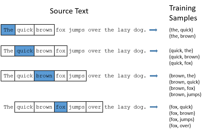
We’ll train the neural network to do this by feeding it word pairs found in our training documents. The below example shows some of the training samples (word pairs) we would take from the sentence “The quick brown fox jumps over the lazy dog.” I’ve used a small window size of 2 just for the example. The word highlighted in blue is the input word.

The network is going to learn the statistics from the number of times each pairing shows up. So, for example, the network is probably going to get many more training samples of (“Soviet”, “Union”) than it is of (“Soviet”, “Sasquatch”). When the training is finished, if you give it the word “Soviet” as input, then it will output a much higher probability for “Union” or “Russia” than it will for “Sasquatch”.

Model Details

So how is this all represented?

First of all, you know you can’t feed a word just as a text string to a neural network, so we need a way to represent the words to the network. To do this, we first build a vocabulary of words from our training documents–let’s say we have a vocabulary of 10,000 unique words.

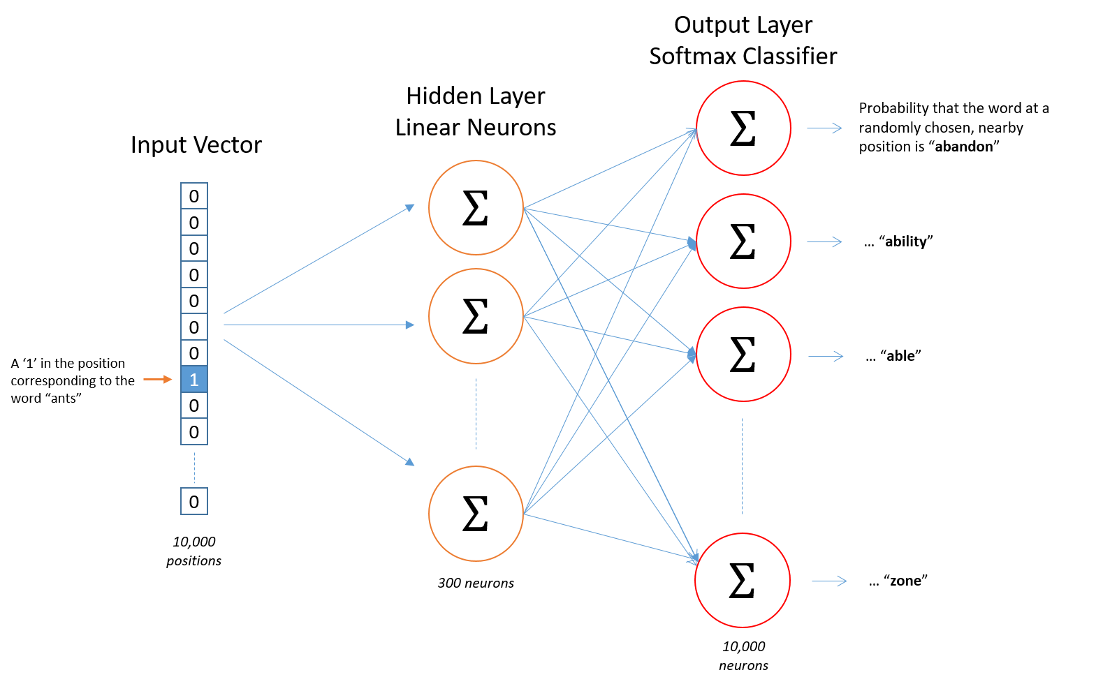
We’re going to represent an input word like “ants” as a one-hot vector. This vector will have 10,000 components (one for every word in our vocabulary) and we’ll place a “1” in the position corresponding to the word “ants”, and 0s in all of the other positions.

The output of the network is a single vector (also with 10,000 components) containing, for every word in our vocabulary, the probability that a randomly selected nearby word is that vocabulary word.

Here’s the architecture of our neural network.

There is no activation function on the hidden layer neurons, but the output neurons use softmax. We’ll come back to this later.

When training this network on word pairs, the input is a one-hot vector representing the input word and the training output is also a one-hot vectorrepresenting the output word. But when you evaluate the trained network on an input word, the output vector will actually be a probability distribution (i.e., a bunch of floating point values, not a one-hot vector).

The Hidden Layer

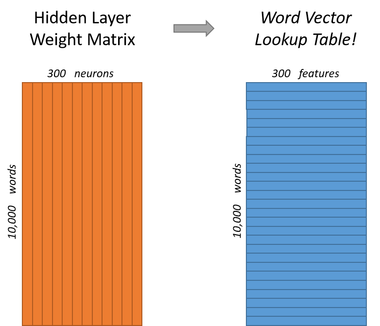
For our example, we’re going to say that we’re learning word vectors with 300 features. So the hidden layer is going to be represented by a weight matrix with 10,000 rows (one for every word in our vocabulary) and 300 columns (one for every hidden neuron).

300 features is what Google used in their published model trained on the Google news dataset (you can download it from here). The number of features is a “hyper parameter” that you would just have to tune to your application (that is, try different values and see what yields the best results).

If you look at the rows of this weight matrix, these are actually what will be our word vectors!

So the end goal of all of this is really just to learn this hidden layer weight matrix – the output layer we’ll just toss when we’re done!

Let’s get back, though, to working through the definition of this model that we’re going to train.

Now, you might be asking yourself–“That one-hot vector is almost all zeros… what’s the effect of that?” If you multiply a 1 x 10,000 one-hot vector by a 10,000 x 300 matrix, it will effectively just select the matrix row corresponding to the “1”. Here’s a small example to give you a visual.

This means that the hidden layer of this model is really just operating as a lookup table. The output of the hidden layer is just the “word vector” for the input word.

The Output Layer

The 1 x 300 word vector for “ants” then gets fed to the output layer. The output layer is a softmax regression classifier. There’s an in-depth tutorial on Softmax Regression here, but the gist of it is that each output neuron (one per word in our vocabulary!) will produce an output between 0 and 1, and the sum of all these output values will add up to 1.

Specifically, each output neuron has a weight vector which it multiplies against the word vector from the hidden layer, then it applies the function exp(x) to the result. Finally, in order to get the outputs to sum up to 1, we divide this result by the sum of the results from all 10,000 output nodes.

Here’s an illustration of calculating the output of the output neuron for the word “car”.

Note that neural network does not know anything about the offset of the output word relative to the input word. It does not learn a different set of probabilities for the word before the input versus the word after. To understand the implication, let’s say that in our training corpus, every single occurrence of the word ‘York’ is preceded by the word ‘New’. That is, at least according to the training data, there is a 100% probability that ‘New’ will be in the vicinity of ‘York’. However, if we take the 10 words in the vicinity of ‘York’ and randomly pick one of them, the probability of it being ‘New’ is not 100%; you may have picked one of the other words in the vicinity.

Intuition

Ok, are you ready for an exciting bit of insight into this network?

If two different words have very similar “contexts” (that is, what words are likely to appear around them), then our model needs to output very similar results for these two words. And one way for the network to output similar context predictions for these two words is if the word vectors are similar. So, if two words have similar contexts, then our network is motivated to learn similar word vectors for these two words! Ta da!

And what does it mean for two words to have similar contexts? I think you could expect that synonyms like “intelligent” and “smart” would have very similar contexts. Or that words that are related, like “engine” and “transmission”, would probably have similar contexts as well.

This can also handle stemming for you – the network will likely learn similar word vectors for the words “ant” and “ants” because these should have similar contexts.

Next Up

You may have noticed that the skip-gram neural network contains a huge number of weights… For our example with 300 features and a vocab of 10,000 words, that’s 3M weights in the hidden layer and output layer each! Training this on a large dataset would be prohibitive, so the word2vec authors introduced a number of tweaks to make training feasible. These are covered in part 2 of this tutorial.

Did you know that the word2vec model can also be applied to non-text data for recommender systems and ad targeting? Instead of learning vectors from a sequence of words, you can learn vectors from a sequence of user actions. Read more about this in my new post here.

Other Resources

I’ve also created a post with links to and descriptions of other word2vec tutorials, papers, and implementations.

Cite

McCormick, C. (2016, April 19). Word2Vec Tutorial - The Skip-Gram Model. Retrieved from http://www.mccormickml.com

Read All
Understanding LSTM Networks

2019-03-13

Henryzhou

reproduction

nlp

转载自：http://colah.github.io/posts/2015-08-Understanding-LSTMs/

Understanding LSTM Networks

Posted on August 27, 2015

Recurrent Neural Networks

Humans don’t start their thinking from scratch every second. As you read this essay, you understand each word based on your understanding of previous words. You don’t throw everything away and start thinking from scratch again. Your thoughts have persistence.

Traditional neural networks can’t do this, and it seems like a major shortcoming. For example, imagine you want to classify what kind of event is happening at every point in a movie. It’s unclear how a traditional neural network could use its reasoning about previous events in the film to inform later ones.

Recurrent neural networks address this issue. They are networks with loops in them, allowing information to persist.

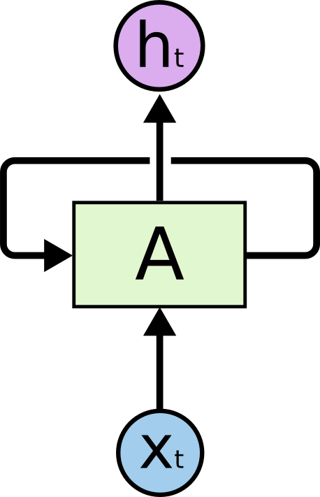
Recurrent Neural Networks have loops.

In the above diagram, a chunk of neural network, AA, looks at some input xtxt and outputs a value htht. A loop allows information to be passed from one step of the network to the next.

These loops make recurrent neural networks seem kind of mysterious. However, if you think a bit more, it turns out that they aren’t all that different than a normal neural network. A recurrent neural network can be thought of as multiple copies of the same network, each passing a message to a successor. Consider what happens if we unroll the loop:

An unrolled recurrent neural network.

This chain-like nature reveals that recurrent neural networks are intimately related to sequences and lists. They’re the natural architecture of neural network to use for such data.

And they certainly are used! In the last few years, there have been incredible success applying RNNs to a variety of problems: speech recognition, language modeling, translation, image captioning… The list goes on. I’ll leave discussion of the amazing feats one can achieve with RNNs to Andrej Karpathy’s excellent blog post, The Unreasonable Effectiveness of Recurrent Neural Networks. But they really are pretty amazing.

Essential to these successes is the use of “LSTMs,” a very special kind of recurrent neural network which works, for many tasks, much much better than the standard version. Almost all exciting results based on recurrent neural networks are achieved with them. It’s these LSTMs that this essay will explore.

The Problem of Long-Term Dependencies

One of the appeals of RNNs is the idea that they might be able to connect previous information to the present task, such as using previous video frames might inform the understanding of the present frame. If RNNs could do this, they’d be extremely useful. But can they? It depends.

Sometimes, we only need to look at recent information to perform the present task. For example, consider a language model trying to predict the next word based on the previous ones. If we are trying to predict the last word in “the clouds are in the sky,” we don’t need any further context – it’s pretty obvious the next word is going to be sky. In such cases, where the gap between the relevant information and the place that it’s needed is small, RNNs can learn to use the past information.

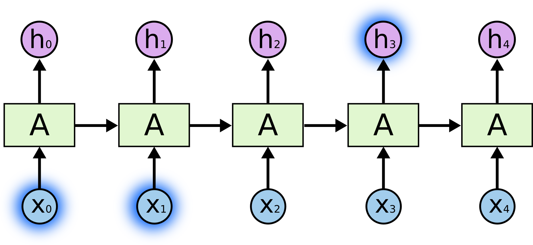
But there are also cases where we need more context. Consider trying to predict the last word in the text “I grew up in France… I speak fluent French.” Recent information suggests that the next word is probably the name of a language, but if we want to narrow down which language, we need the context of France, from further back. It’s entirely possible for the gap between the relevant information and the point where it is needed to become very large.

Unfortunately, as that gap grows, RNNs become unable to learn to connect the information.

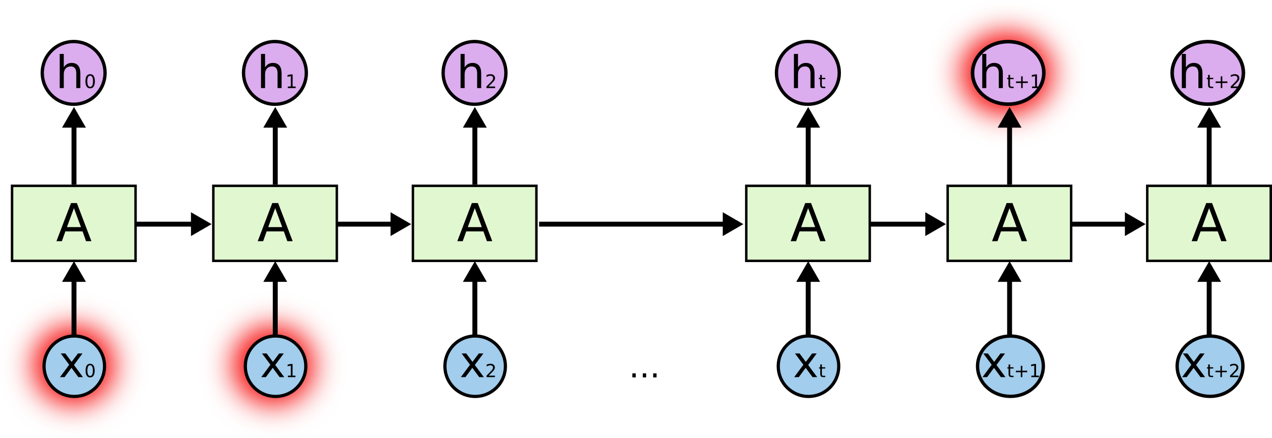
In theory, RNNs are absolutely capable of handling such “long-term dependencies.” A human could carefully pick parameters for them to solve toy problems of this form. Sadly, in practice, RNNs don’t seem to be able to learn them. The problem was explored in depth by [Hochreiter (1991) German] and Bengio, et al. (1994), who found some pretty fundamental reasons why it might be difficult.

Thankfully, LSTMs don’t have this problem!

LSTM Networks

Long Short Term Memory networks – usually just called “LSTMs” – are a special kind of RNN, capable of learning long-term dependencies. They were introduced by Hochreiter & Schmidhuber (1997), and were refined and popularized by many people in following work.1 They work tremendously well on a large variety of problems, and are now widely used.

LSTMs are explicitly designed to avoid the long-term dependency problem. Remembering information for long periods of time is practically their default behavior, not something they struggle to learn!

All recurrent neural networks have the form of a chain of repeating modules of neural network. In standard RNNs, this repeating module will have a very simple structure, such as a single tanh layer.

Read All
pytorch中rnn的使用

2019-03-13

Henryzhou

reproduction

pytorch
转载自：https://github.com/zergtant/pytorch-handbook/blob/master/chapter2/2.5-rnn.ipynb
```
import torch
torch.__version__
```
Read All

使用pytorch进行fine-tune

2019-03-13

Henryzhou

reproduction

pytorch

%matplotlib inline
import torch,os,torchvision
import torch.nn as nn
import torch.nn.functional as F
import pandas as pd
import numpy as np
import matplotlib.pyplot as plt
from torch.utils.data import DataLoader, Dataset
from torchvision import datasets, models, transforms
from PIL import Image
from sklearn.model_selection import StratifiedShuffleSplit
torch.__version__

Read All

深入解析torch.nn

2019-03-12

Henryzhou

reproduction

pytorch
转载自：https://blog.csdn.net/weixin_36811328/article/details/87905208

原文地址：WHAT IS TORCH.NN REALLY? 本人英语学渣，如有错误请及时指出以便更正，使用的源码可点击原文地址进行下载。

pytorch提供了许多优雅的类和模块帮助我们构建与训练网络，比如 torch.nn, torch.optim,Dataset等。为了充分利用这些模块的功能，灵活操作它们解决各种不同的问题，我们需要更好地理解当我们调用这些模块时它们到底干了些什么，为此，我们首先不调用这些模块实现MNIST手写字识别，仅使用最基本的 pytorch 张量函数。然后，我们逐渐增加 torch.nn, torch.optim, Dataset, or DataLoader,具体地展示每个模块具体干了些什么，展示这些模块是怎样使代码变得更加优雅灵活。 此教程适用范围：熟悉pytorch的张量操作

加载 MNIST 数据集

我们使用经典的 MNIST 数据集，一个包含了0-9数字的二值图像库。

还会用到 pathlib 库用于目录操作，一个python3自带的标准库。使用 requests 下载数据集。当用到一个模块时才会进行导入，而不会一开始全部导入，以便更好地理解每个步骤。
```
from pathlib import Path
import requests

DATA_PATH = Path('data')
PATH = DATA_PATH / "mnist"

PATH.mkdir(parents=True,exit_ok=True)

URL = "http://deeplearning.net/data/mnist/"
FILENAME = "mnist.pkl.gz"

if not (PATH / FILENAME).exists():
	content = requests.get(URL + FILENAME).content
	(PATH / FILENAME).open("wb").write(content)
1234567891011121314
```
该数据集采用numpy数组格式，并使用pickle存储，pickle是一种特定于python的格式，用于序列化数据。
```
import pickle
import gzip

with gzip.open((PATH / FILENAME).as_posix(),"rb") as f:
	((x_train,y_train),(x_valid,y_valid),_) = pickle.load(f,encoding="latin-1")
12345
```
每张训练图片分辨率为 28x28，被存储为 784(=28x28) 的一行。我们输出看一下数据，首先需要转换回 28x28的图像。
```
form matplotlib import pyplot
import numpy as np

pyplot.imshow(x_train[0].reshape((28,28)),cmap="gray")
print(x_train.shape)
12345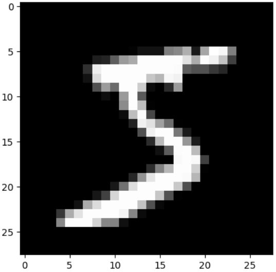
```
out:
```
(50000,784)
1
```
PyTorch使用 torch.tensor ，所以我们需要对numpy类型数据进行转换
```
import torch
x_train,y_train,x_valid,y_valid = map(
	torch.tensor,(x_train,y_train,x_valid,y_valid)
	)
n,c = x_train.shape
x_train,x_train.shape,y_train.min(),y_train.max()
print(x_train,y_train)
print(x_train.shape)
print(y_train.min(),y_train.max())
123456789
```
从头创建神经网络（不使用torch.nn）

让我们仅仅使用 pytorch 中的张量操作来创建模型，假设你已经熟悉神经网络的基础知识（不熟悉请参考corse.fast.ai ）

pytorch提供了很多创建张量的操作，我们将用这些方法来初始化权值weights和偏置 bais来创建一个线性模型。这些只是常规张量，有一个非常特别的补充：我们告诉PyTorch这些张量需要支持求导(requires_grad=True)。这样PyTorch将记录在张量上完成的所有操作，以便它可以在反向传播过程中自动计算梯度！

对于权值weights，我们再初始化之后再设置 requires_grad,因为我们不想这一步包含在梯度的计算中（注：pytorch中以 _ 结尾的操作都是在原变量中(in-place)执行的）
```
import math

weights = torch.randn(780,10) / math.sqrt(784)
weights.requires_grad_()
bias = torch.zeros(10, requires_grad=True)
12345
```
多亏了pytorch的自动求导功能，我们可以使用python的所有标准函数来构建模型。我们这儿利用矩阵乘法，加法来构建线性模型。我们编写 log_softmax函数作为激活函数。虽然pytorch提供了大量写好的损失函数，激活函数，你依然可以自由地编写自己的函数替代它们。 pytorch 甚至支持创建自己的 GPU函数或者CPU矢量函数。
```
def log_softmax(x):
	return x - x.exp().sum(-1).log().unsqueeze(-1)

def model(xb):
	return log_softmax(xb @ weights + bias)           # python的广播机制
12345
```
上面的 @ 符号表示向量的点乘，接下来我们会调用一批数据（batch，64张图片）输入此模型。
```
bs = 64 					# batch size
xb = x_train[0:bs]    		# a mini-batch from x
preds = model(xb)   		# predictions
print(preds[0],preds.shape)
1234
```
out:
```
tensor([-2.4513, -2.5024, -2.0599, -3.1052, -3.2918, -2.2665, -1.9007, -2.2588,
        -2.0149, -2.0287], grad_fn=<SelectBackward>) torch.Size([64, 10])
12
```
正如我们看到的，preds 张量不仅包含了一组张量，还包含了求导函数。反向传播的时候会用到此函数。让我们使用标准的python语句接着来实现 negative log likelihood loss 损失函数（译者加：也被称为交叉熵损失函数）：
```
def nll(input,target):
	return -input[range(target.shape[0]),target].mean()

loss_func = nll
1234
```
现在用我们的损失函数来检查我们随机初始化的模型，待会就能看到再反向传播之后是否会改善模型性能。
```
yb = y_train[0:bs]
print(loss_func(preds,yb))
12
```
out:
```
tensor(2.3620, grad_fn=<NegBackward>)
1
```
接下来定义一个计算准确度的函数
```
def accuracy(out,yb)：
	preds = torch.argmax(out,dim=1)           # 得到最大值的索引
	return (preds == yb).float().mean()
123
```
检查模型的准确度：
```
print(accuracy(preds, yb))
1
```
out:
```
tensor(0.0938)
1
```
现在我们开始循环训练模型，每一步我们执行以下操作：
- 选择一批数据（a batch）
- 使用模型进行预测
- 计算损失函数
- 反向传播更新参数 weights 和 bias
我们现在使用 torch.no_grad() 更新参数，以避免参数更新过程被记录入求导函数中。

然后我们清零导数，以便开始下一轮循环，否则导数会在原来的基础上累加，而非替代原来的数
```
from IPython.core.debugger import set_trace

lr = 0.5  # learning rate
epochs = 2  # how many epochs to train for

for epoch in range(epochs):
    for i in range((n - 1) // bs + 1):
        #         set_trace()
        start_i = i * bs
        end_i = start_i + bs
        xb = x_train[start_i:end_i]
        yb = y_train[start_i:end_i]
        pred = model(xb)
        loss = loss_func(pred, yb)

        loss.backward()
        with torch.no_grad():
            weights -= weights.grad * lr
            bias -= bias.grad * lr
            weights.grad.zero_()
            bias.grad.zero_()
123456789101112131415161718192021
```
目前为止，我们从头创建一个迷你版的神经网络

让我们来检查一下损失和准确率，并于迭代更新参数之前进行比较，我们期望得到更小的损失于更高的准确率。
```
print(loss_func(model(xb), yb), accuracy(model(xb), yb))
1
```
out:
```
tensor(0.0822, grad_fn=<NegBackward>) tensor(1.)
1
```
使用 torch.nn.functional 简化代码

现在我们使用torch.nn.functional重构之前的代码，这样会使代码变得更加简洁与灵活，更易理解。

首先最简单的一步是，用 torch.nn.functional( 为了方便后面统一称作F) 中带有的损失函数来代替我们自己编写的函数，使得代码变得更简短。这些函数都包包含于模块 torch.nn里面，除了大量的损失函数与激活函数，里面还包含了大量用于构建网络的函数。

如果我们的网络中使用 negative log likelihood loss 作为损失函数， log softmax activation 作为激活函数（即我们上面实现的损失函数与激活函数）。在pytorch中我们直接使用函数 F.cross_entropy 便可实现上面两个函数的功能。所以我们可以用此函数代替上面实现的激活函数与损失函数。
```
import torch.nn.functional as F

loss_func = F.cross_entropy

def model(xb):
	return xb @ weights + bias
123456
```
让我测试一下是否和上面自己实现的函数效果一致：
```
print(loss_func(model))
1
```
out:
```
tensor(0.0822, grad_fn=<NllLossBackward>) tensor(1.)
1
```
引入 nn.Module 重构代码

接下来我们引入 nn.Module和nn.Parameter 改进代码。我们创建 nn.Module的子类。这个例子中我们创建一个包含权重，偏置，以及包含前向传播的类。nn.Module含有许多的属性与方法可供调用（比如： .parameters .zero_grad()）
```
from torch import nn

class Mnist_Logistic(nn.Module):
	def __init__(self):
		super().__init__()
		sefl.weights = nn.Parameter(torch.randn(784,10)/math.sqrt(784))
		self.bias = nn.Parameter(torch.zeros(10))

	def forward(self,xb):
		return xb @ self.weights + self.bias
12345678910
```
接下来实例化我们的模型：
```
model = Mnist_Logistic()
1
```
现在我们可以和之前一样使用损失函数了。注意：nn.Module 对象可以像函数一样调用，但实际上是自动调用了对象内部的函数 forward
```
print(loss_func(model(xb),yb))
1
```
out:
```
tensor(2.2082, grad_fn=<NllLossBackward>)
1
```
在之前，我们必须进行如下得操作对权重，偏置进行更新，梯度清零：
```
with torch.no_grad():
	weights -= weights.grad * lr
	bias -= bias.grad * lr
	weights.grad.zero_()
	bias.grad.zero_()
12345
```
现在我们可以充分利用 nn.Module 的方法属性更简单地完成这些操作，如下所示：
```
with torch.no_grad():
	for p in model.parameters(): p -= p.grad * lr
	model.zero_grad()
123
```
现在我们将整个训练过程写进函数 fit中。
```
def fit():
	for epoch in range(epoches):
		for i in range((n - 1) // bs + 1):
			start_i = i * bs
			end_i = start_i + bs
			xb = x_train[start_i:end_i]
			yb = y_train[start_i:end_i]
			pred = model(xb)
			loss = loss_func(pred,yb)
		
			loss.backward()
			with torch.no_grad():
				for p in model.parameters(): p -= p.grad * lr
				model.zero_grad()
fit()
123456789101112131415
```
让我们再一次确认损失情况：
```
print(loss_func(model(xb),yb))
1
```
out:
```
tensor(0.0812, grad_fn=<NllLossBackward>)
1
```
引入 nn.Linear 重构代码

比起手动定义权重与偏置，并且使用 self.weights和 self.bias 来计算 xb @ self.weights + self.bias的方式，我们可以使用pytorch中的 nn.Linear来定义线性层，他自动为我们实现以上权重参数的定义以及计算的过程。除了线性模型之外，pytorch还有一系列的其它网络层供我们使用，大大简化了我们的编程过程。
```
class Mnist_Logistic(nn.Module):
	def __init__(self):
		super().__init__()
		self.lin = nn.Linear(784,10)

	def forward(self,xb):
		return self.lin(xb)
1234567
```
同上面一样实例化模型，计算损失
```
model = Mnist_Logistic()
print(loss_func(model(xb),yb))
12
```
out:
```
tensor(2.2731, grad_fn=<NllLossBackward>)
1
```
训练，并查看训练之后的损失
```
fit()

print(loss_func(model(xb), yb))
123
```
out:
```
tensor(0.0820, grad_fn=<NllLossBackward>)
1
```
引入 optim 重构代码

接下来使用torch.optim改进训练过程，而不用手动更新参数

之前的手动优化过程如下：
```
with torch.no_grad():
	for p in model.parameters(): p -= p.grad * lr
	model.zero_grad()
123
```
使用如下代码替代手动的参数更新：
```
opt.step()
# optim.zero_grad() resets the gradient to 0 and we need to call it 
# before computing the gradient for the next minibatch.
opt.zero_grad() 
1234
```
结合之前的完整跟新代码如下：
```
from torch import optim

def get_model():
	model = Mnist_Logistic()
	return model, optim.SGD(model.parameters(),lr=lr)

model, opt = get_model()
print(loss_func(model(xb),yb))

for epoch in range(epoches):
	for i in range((n-1)//bs + 1):
		start_i = i *bs
		end_i = start_i + bs
		xb = x_train[start_i:end_i]
		yb = y_train[start_i:end_i]
		pred = model(xb)
		loss = loss_func(pred,yb)

		loss.backward()
		opt.step()
		opt.zero_grad()

print(loss_func(model(xb),yb))
1234567891011121314151617181920212223
```
out:
```
tensor(2.3785, grad_fn=<NllLossBackward>)
tensor(0.0802, grad_fn=<NllLossBackward>)
12
```
引入 Dataset 处理数据

pytorch定义了 Dataset 类，其中主要包含了 __len__ 函数与 __getitem__函数。此教程以创建 FacialLandmarkDataset 为例详细地介绍了Dataset类的使用。

pytorch的 TensorDataset 是一个包含张量的数据集。通过定义长度索引等方式，使我们更好地利用索引，切片等方法迭代数据。这会让我们很容易地在一行代码中获取我们地数据。
```
form torch.utils.data import TensorDataset
1
```
x_train y_train可以被组合进一个TensorDataset中，这会使得迭代切片更加简单。
```
train_ds = TensorDataset(x_train,y_train)
1
```
之前我们获取数据的方法如下：
```
xb = x_train[start_i:end_i]
yb = y_train[start_i:end_i]
12
```
现在我们可以使用更简单的方法：
```
xb,yb = train_ds[i*bs : i*bs +bs]
1
model, opt = get_model()

for epoch in range(epochs):
    for i in range((n - 1) // bs + 1):
        xb, yb = train_ds[i * bs: i * bs + bs]
        pred = model(xb)
        loss = loss_func(pred, yb)

        loss.backward()
        opt.step()
        opt.zero_grad()

print(loss_func(model(xb), yb))
12345678910111213
```
out:
```
tensor(0.0817, grad_fn=<NllLossBackward>)
1
```
引入DataLoader加载数据

DataLoader 用于批量加载数据，你可以用他来加载任何来自 Dataset的数据，它使得数据的批量加载十分容易。
```
from torch.utils.data import DataLoader

train_ds = TensorDataset(x_train,y_train)
train_dl = DataLoader(train_ds, batch_size=bs)
1234
```
之前我们读取数据的方式：
```
for i in range((n-1)//bs + 1):
    xb,yb = train_ds[i*bs : i*bs+bs]
    pred = model(xb)
123
```
现在使用dataloader加载数据：
```
for xb,yb in train_dl:
    pred = model(xb)
12
model, opt = get_model()

for epoch in range(epochs):
    for xb, yb in train_dl:
        pred = model(xb)
        loss = loss_func(pred, yb)

        loss.backward()
        opt.step()
        opt.zero_grad()

print(loss_func(model(xb), yb))
123456789101112
```
out:
```
tensor(0.0817, grad_fn=<NllLossBackward>)
1
```
目前为止训练模型部分我们就已经完成了，通过使用nn.Module, nn.Parameter, DataLoader, 我们的训练模型以及得到了很大的改进。接下来让我们开始模型的测试部分。

添加测试集

在前一部分，我们尝试了使用训练集训练网络。实际工作中，我们还会使用测试集来观察训练的模型是否过拟合。

打乱数据的分布有助于减小每一批(batch)数据间的关联，有利于模型的泛化。但对于测试集来说，是否打乱数据对结果并没有影响，反而会花费多余的时间，所以我们没有必要打乱测试集的数据。
```
train_ds = TensorDataset(x_train, y_train)
train_dl = DataLoader(train_ds, batch_size=bs, shuffle=True)

valid_ds = TensorDataset(x_valid, y_valid)
valid_dl = DataLoader(valid_ds, batch_size = bs*2)
12345
```
在每训练完一轮数据（epoch）后我们输出测试得到的损失值。 (注：如下代码中，我们调用model.train()和model.eval表示进入训练模式与测试模式，以保证模型运行的准确性)
```
model,opt = get_model()

for epoch in range(epoches):
	model.train()
	for xb, yb in train_dl:
		pred = model(xb)
		loss = loss_func(pred, yb)
		
		loss.backward()
		opt.step()
		opt.zero_grad()

	model.eval()
	with torch.no_grad():
		valid_loss = sum(loss_func(model(xb), yb) for xb, yb in valid_dl)

	print(epoch, valid_loss / len(valid_dl))
1234567891011121314151617
```
out:
```
0 tensor(0.3456)
1 tensor(0.2988)
12
```
创建 fit() 和 get_data() 优化代码

我们再继续做一点改进。因为我们再计算训练损失和验证损失时执行了两次相同的操作，所以我们用一个计算每一个batch损失的函数封装这部分代码。

我们为训练集添加优化器，并执行反向传播。对于训练集我们不添加优化器，当然也不会执行反向传播。
```
def loss_batch(model, loss_func, xb , yb, opt=None):
	loss = loss_func(model(xb),yb)

	if opt is not None:
		loss.backward()
		opt.step()
		opt.zero_grad()
	
	return loss.item(), len(xb)
123456789
```
fit执行每一个epoch过程中训练和验证的必要操作
```
import numpy as np 

def fit(epochs, model, loss_func, opt, train_dl, valid_dl):
	for epoch in range(epochs):
		model.train()
		for xb, yb in train_dl:
			loss_batch(model, loss_func, xb, yb, opt)
		
		model.eval()
		with torch.no_grad():
			losses, nums = zip(
				*[loss_batch(model, loss_func, xb, yb) for xb, yb in valid_dl]
			)
		val_loss = np.sum(np.sum(np.multiply(losses, nums)). np.sum(nums))

		print(epoch, val_loss)
12345678910111213141516
```
现在，获取数据加载模型进行训练的整个过程只需要三行代码便能实现了
```
train_dl, valid_dl = get_data(train_ds, valid_ds, bs)
model, opt = get_model()
fit(epoches, model, loss_func, opt, train_dl, valid_dl)
123
```
out:
```
0 0.2961075816631317
1 0.28558296990394594
12
```
我们可以用这简单的三行代码训练各种模型。下面让我们看看怎么用它训练一个卷积神经网络。

使用卷积神经网络

现在我们用三个卷积层来构造我们的卷积网络。因为之前的实现的函数都没有假定模型形式，这儿我们依然可以使用它们而不需要任何修改。

我们pytorch预定义的Conv2d类来构建我们的卷积层。我们模型有三层，每一层卷积之后都跟一个 ReLU，然后跟一个平均池化层。
```
class Mnist_CNN(nn.Module):
	def __init__(self):
		super().__init__()
		self.conv1 = nn.Conv2d(1,16,kernel_size=3,stride=2,padding=1)
		self.conv2 = nn.Conv2d(16,16,kernel_size=3,stride=2,padding=1)
		self.conv3 = nn.Conv2d(16,10,kernel_size=3,stride=2,padding=1)

	def forward(self, xb):
		xb = xb.view(-1,1,28,28)
		xb = F.relu(self.conv1(xb))
		xb = F.relu(self.conv2(xb))
		xb = F.relu(self.conv3(xb))
		xb = F.avg_pool2d(xb,4)
		return xb.view(-1, xb.size(1))

lr = 0.1
12345678910111213141516
```
动量momentum是随机梯度下降的一个参数，它考虑到了之前的梯度值使得训练更快。
```
model = Mnist_CNN()
opt = optim.SGD(model.parameters(), lr=lr, momentum=0.9)

fit(epochs, model, loss_func, opt, train_dl, valid_dl)
1234
```
out:
```
0 0.3829730714321136
1 0.2258522843360901
12
```
使用 nn.Sequential 搭建网络

torch.nn还有另外一个方便的类可以简化我们的代码：Sequential, 一个Sequential对象
```
class Lambda(nn.Module):
	def __init__(self, func):
		super().__init__()
		self.func = func

	def forward(self, x):
		return self.func(x)

def preprocess(x):
	return x.view(-1, 1, 28, 28)
12345678910
```
Sequential是一种简化代码的好方法。一个Sequential对象按顺序执行包含在内的每一个module，使用它可以很方便地建立一个网络。

为了更好地使用Sequential模块，我们需要自定义 pytorch中没实现地module。例如pytorch中没有自带改变张量形状地层，我们创建 Lambda层，以便在Sequential中调用。
```
model = nn.Sequential(
    Lambda(preprocess),
    nn.Conv2d(1, 16, kernel_size=3, stride=2, padding=1),
    nn.ReLU(),
    nn.Conv2d(16, 16, kernel_size=3, stride=2, padding=1),
    nn.ReLU(),
    nn.Conv2d(16, 10, kernel_size=3, stride=2, padding=1),
    nn.ReLU(),
    nn.AvgPool2d(4),
    Lambda(lambda x: x.view(x.size(0), -1)),
)

opt = optim.SGD(model.parameters(), lr=lr, momentum=0.9)

fit(epochs, model, loss_func, opt, train_dl, valid_dl)
123456789101112131415
```
out:
```
0 0.32739396529197695
1 0.25574398956298827
12
```
简易的DataLoader

我们的网络以及足够精简了，但是只能适用于MNIST数据集，因为
- 网络默认输入为 28x28 的张量
- 网络默认最后一个卷积层大小为 4x4 （因为我们的池化层大小为4x4）
现在我们去除这两个假设，使得网络可以适用于所有的二维图像。首先我们移除最初的 Lambda层，用数据预处理层替代。
```
def preprocess(x, y):
	return x.view(-1, 1, 28, 28), y

class WrappedDataLoader:
	def __init__(self, dl, func):
		self.dl = dl
		self.func = func

	def __len__(self):
		return len(self.dl)

	def __iter__(self):
		batches = iter(self.dl)
		for b in batches:
			yield (self.func(*b))

train_dl, valid_dl = get_data(train_ds, valid_ds, bs)
train_dl = WrappedDataLoader(train_dl, preprocess)
valid_dl = WrappedDataLoader(valid_dl, preprocess)
12345678910111213141516171819
```
然后，我们使用nn.AdaptiveAvgPool2d代替nn.AvgPool2d。它允许我们自定义输出张量的维度，而于输入的张量无关。这样我们的网络便可以适用于各种size的网络。
```
model = nn.Sequential(
	nn.Conv2d(1, 16, kernal_size=3, stride=2, padding=1),
	nn.ReLU(),
	nn.Conv2d(16, 16, kernel_size=3, stride=2, padding=1),
	nn.ReLU(),
	nn.Conv2d(16, 10, kernel_size=3, stride=2, padding=1),
    nn.ReLU(),
    nn.AdaptiveAvgPool2d(1),
    Lambda(lambda x: x.view(x.size(0), -1)),
	)

opt = optim.SGD(model.parameters(), lr=lr, momentum=0.9)
123456789101112
```
out:
```
0 0.32888883714675904
1 0.31000419993400574
12
```
使用GPU

如果你的电脑有支持CUDA的GPU（你可以很方便地以 0.5美元/小时的价格租到支持的云服务器），便可以使用GPU加速训练过程。首先检测设备是否正常支持GPU:
```
print(torch.cuda.is_available())
1
```
out:
```
Ture
1
```
接着创建一个设备对象：
```
dev = torch.device(
	"cuda") if torch.cuda.is_available() else torch.device("cpu")
12
```
更新 preprocess(x,y)把数据移到GPU:
```
def preprocess(x, y):
	return x.view(-1, 1, 28, 28).to(dev), y.to(device)

train_dl, valid_dl = get_data(train_ds, valid_ds, bs)
train_dl = WrappedDataLoader(train_dl, preprocess)
valid_dl = WrappedDataLoader(valid_dl, preprocess)
123456
```
最后移动网络模型到GPU：
```
model.to(dev)
opt = optim.SGD(model.parameters(),lr=lr, momentum=0.9)
12
```
进行训练，能发现速度快了很多：
```
fit(epochs, model, loss_func, opt, train_dl, valid_dl)
1
```
out:
```
0 0.21190375366210937
1 0.18018000435829162
12
```
总结

我们现在得到了一个通用的数据加载和模型训练方法，我们可以在pytorch种用这种方法训练大多的模型。想知道训练一个模型有多简单，回顾一下本次的代码便可以了。

当然，除此之外本篇内容还有很多需求没有讲到，比如数据增强，超参调试，数据监控(monitoring training),迁移学习等。这些特点都以与本篇教程相似的设计方法包含于 fastai库中。

本篇教程开头我们承诺将会通过例程解释 torch.nn torch.optim Dataset DataLoader等模块，下面我们就这些模型进行总结。
- torch.nn
  - Module: 创建一个可以像函数一样调用地对象，包含了网络的各种状态，可以使用parameter方便地获取模型地参数，并有清零梯度，循环更新参数等功能。
  - Parameter: 将模型中需要更新的参数全部打包，方便反向传播过程中进行更新。有 requires_grad属性的参数才会被更新。
  - functional：通常导入为F，包含了许多激活函数，损失函数等。
- torch.optim: 包含了很多诸如SGD一样的优化器，用来在反向传播中跟新参数
- Dataset: 一个带有 __len__ __getitem__等函数的抽象接口。里面包含了 TensorDataset等类。
- DataLoader: 输入任意的 Dataset 并按批(batch)迭代输出数据。
Read All

爬虫环境安装

2019-03-11

Henryzhou

notes

spider

spider Note

python环境安装

python3.7

请求库的安装

请求库requests的安装：conda install requests -n spider
自动化测试工具Senlenium的安装：conda install selenium -n spider

senlenium驱动chrome浏览器工具chromedriver添加到PATH中：

在~/.bashrc最后添加：PATH=/home/henry/opt:$PATH
source ~/.bashrc

使用phantomJS实现后台的浏览器控制

下载phantomJS，并且将其路径添加到系统变量中

安装异步web请求库aiohttp
```
conda install aiohttp -n spider
```

解析库的安装

lxml的安装，支持HTML、XML的解析，支持XPath解析方式
```
conda install lxml -n spider
```
beautifulsoup4的安装，其依赖lxml
```
conda install beautifulsoup4 -n spider
```
pyquery的安装
```
conda install pyquery -n spider
```

安装验证码识别工具tesseract

sudo apt install -y tesseract-ocr libtesseract-dev libleptonica-dev
conda activate spider
pip install tesserocr pillow

数据库的安装

mysql的安装

sudo apt update
sudo apt install -y mysql-server mysql-client
#mysql启动、关闭、重启命令
#sudo service mysql start
#sudo service mysql stop
#sudo service mysql restart

mysql5.7以上不会有密码设置过程，需要手动配置
$ mysql -u debian-sys-maint -p
#密码在/etc/mysql/debian.cnf文件中可查看(V3XKquzHqnW18GWc)，在mysql命令行中执行下列语句
  
show databases；
use mysql;
update user set authentication_string=PASSWORD("zhou") where user='root';
update user set plugin="mysql_native_password";
flush privileges;
quit;

#完全卸载mysql的方法
sudo apt purge mysql-*
sudo rm -rf /etc/mysql/ /var/lib/mysql
sudo apt autoremove

安装redis
```
sudo apt install redis-server
```

存储库的安装

安装pymysql存储库以使用python和mysql交互
```
conda install pymysql -n spider
```
安装redis_py
```
conda install redis -n spider
```

Web库的安装

安装Flask web库来搭建一些API接口，供爬虫使用，后面会利用Flask+Redis维护动态代理池和Cookies池
```
conda install tornado -n spider
```
安装tornado，后面会使用tornado+redis来搭建一个ADSL拨号代理池

Read All

6/9

Welcome to Henry's Blog!

Word2Vec Tutorial

Word2Vec Tutorial - The Skip-Gram Model

The Model

The Fake Task

Model Details

The Hidden Layer

The Output Layer

Intuition

Next Up

Other Resources

Cite

Understanding LSTM Networks

Understanding LSTM Networks

Recurrent Neural Networks

The Problem of Long-Term Dependencies

LSTM Networks

pytorch中rnn的使用

使用pytorch进行fine-tune

深入解析torch.nn

加载 MNIST 数据集

从头创建神经网络（不使用torch.nn）

使用 torch.nn.functional 简化代码

引入 nn.Module 重构代码

引入 nn.Linear 重构代码

引入 optim 重构代码

引入 Dataset 处理数据

引入DataLoader加载数据

添加测试集

创建 fit() 和 get_data() 优化代码

使用卷积神经网络

使用 nn.Sequential 搭建网络

简易的DataLoader

使用GPU

总结

爬虫环境安装

spider Note

python环境安装

请求库的安装

解析库的安装

数据库的安装

存储库的安装

Web库的安装